A Databricks bill looks simple until you try to forecast the next one. For many teams, Databricks pricing feels predictable in a pilot and much less so once ETL, BI, notebooks, and AI work all land on the same platform.
The reason is straightforward. You’re not buying one flat product. You’re paying for platform usage, compute behavior, and cloud infrastructure at the same time.
If you need a practical view for 2026, start with how the bill is built, then map each workload to the right compute type.
How Databricks pricing is built
Databricks charges in DBUs, short for Databricks Units. A DBU is a usage measure for Databricks compute and platform services. In plain terms, the platform tracks how much processing capacity your workload consumes, bills it at a rate tied to the workload type and edition, and then adds the underlying cloud bill unless you use serverless.
The official Databricks pricing page still frames the model as pay as you go, billed per second, with no upfront fee. That sounds simple, but the bill has two layers for most classic deployments. First comes the DBU charge. Then come AWS, Azure, or GCP costs for VMs, storage, networking, and related services.
Total monthly cost usually works like this: DBUs consumed x DBU rate, plus cloud infrastructure.
That split matters because teams often track only one side. A platform lead may watch DBUs while finance sees a larger cloud number. Meanwhile, data scientists may keep an interactive cluster alive all afternoon without noticing either line item.
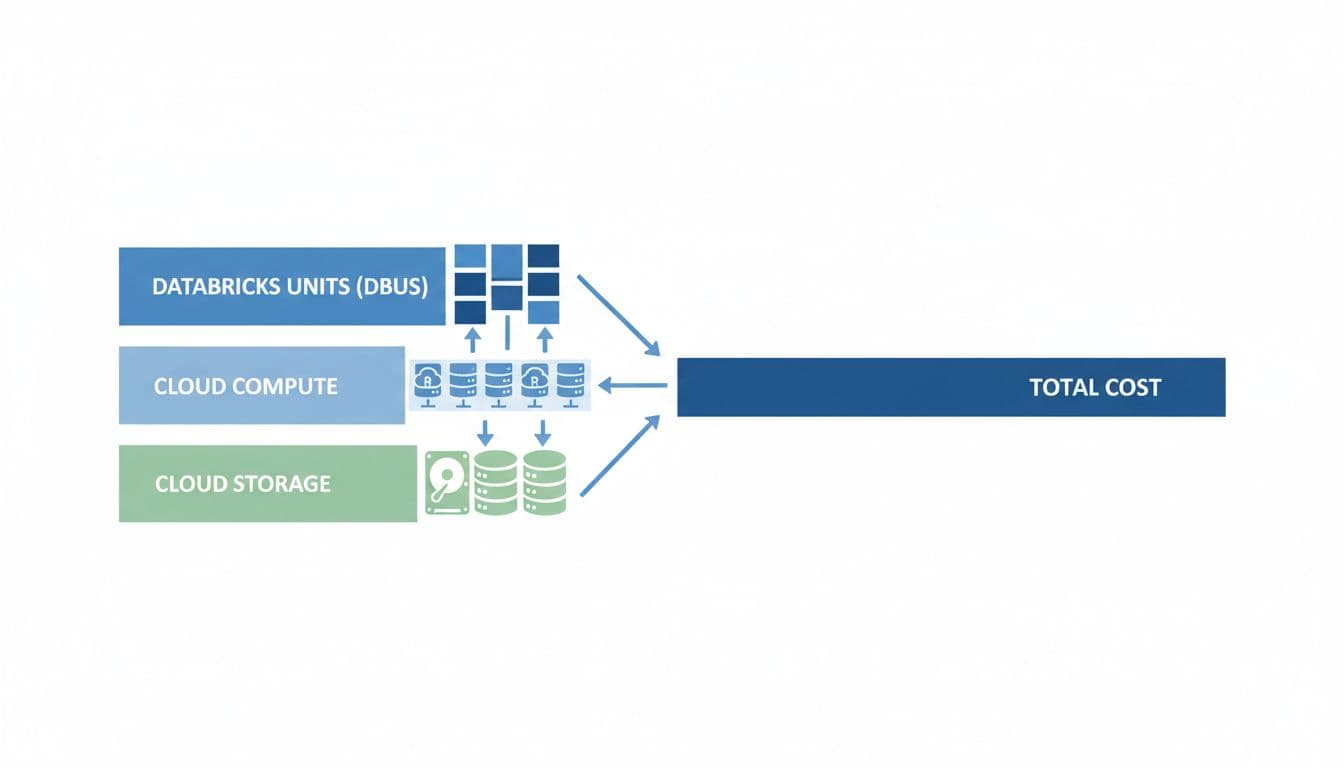
Serverless changes the structure. In supported areas, Databricks bundles the cloud compute into the service price, so the rate is usually higher but easier to read. That trade-off is attractive for teams that want less cluster management and faster start-up. Still, simpler billing doesn’t always mean lower total spend.
For procurement teams, one more layer matters. Databricks offers committed-use discounts, and Microsoft lists pre-purchased Azure Databricks capacity with potential savings on the Azure Databricks pricing page. The discount only helps when usage is steady enough to earn it.
The variables that change your bill the fastest
Four things drive most cost swings: workload type, edition, cloud, and region.
Workload type is the biggest lever. A scheduled ETL pipeline, an analyst SQL warehouse, and a shared notebook cluster don’t use the same SKU or DBU rate. That’s why two teams can process similar data volumes yet produce very different invoices.
Edition is next. More governance, security, and enterprise controls usually mean a higher platform rate. On Azure, the packaging can differ from AWS and GCP. Databricks notes on its interactive workload pricing page that Azure Databricks is billed and supported by Microsoft, and the tier mapping does not always line up one to one with the other clouds.
Cloud choice also affects both halves of the bill. Public examples in 2026 often show AWS as the lowest-cost starting point, GCP close behind, and Azure higher in some cases. Yet the gap isn’t only a DBU issue. VM pricing, reserved capacity, regional discounts, network egress, and storage behavior can change the result.
Region pushes the same workload up or down again. A team in US East may see a lower unit rate than a team in Mumbai or another higher-cost region. That is why flat claims like “Databricks costs X per month” rarely help. Without the cloud, region, edition, and workload mix, the number doesn’t travel well.
One more point often gets missed. DBUs are not a simple synonym for node hours. Consumption depends on cluster type, instance family, and how Databricks classifies the workload. So a cost model built only on “number of nodes x hours” will usually miss the mark.
What common workload types cost in 2026
The table below shows how pricing usually looks across the workloads most lakehouse and AI teams run.
| Workload type | Common use | Typical cost pattern | Public 2026 examples* | Main risk |
|---|---|---|---|---|
| Jobs Compute | Scheduled ETL, batch pipelines, production transforms | Lowest DBU tier in many setups, plus cloud infra | Around $0.07 AWS Standard, around $0.15 AWS Premium | Teams run the same job on pricier interactive compute |
| All-Purpose Compute | Shared notebooks, ad hoc analysis, ML development | Higher DBU rate, plus cloud infra | Around $0.40 AWS Standard, around $0.55 AWS Premium | Idle clusters and long-lived dev environments |
| SQL Warehouse | BI dashboards, analyst queries, semantic workloads | Mid-range DBU rate, separate infra unless serverless | Around $0.22 in public examples | Oversized warehouses and always-on settings |
| Serverless | Managed SQL, jobs, notebooks in supported areas | Higher unit price, infra bundled into service | Around $0.75 AWS Premium, around $0.95 Azure in public examples | Convenience hides query waste and weak controls |
*Examples reflect public 2026 pricing references and market guides, not a universal quote. Verify with your cloud, region, edition, and current SKU pages.
Jobs Compute is usually the best value for production data engineering. If a task runs on a schedule and doesn’t need an always-available cluster, jobs pricing is hard to beat. That’s why moving production ETL off All-Purpose clusters is one of the fastest ways to cut spend.
All-Purpose compute is where data science and notebook-driven work often lives. It supports interactive exploration well, but it’s also where unused hours pile up. Five people sharing a cluster can be efficient. Five mostly idle clusters are not.
SQL workloads fit best on Databricks SQL pricing rather than general notebook compute. BI tools, dashboards, and repeated analyst queries tend to run cleaner there. In many cases, Photon-backed SQL warehouses finish work faster, which lowers cost per completed query even if the DBU rate looks similar.
Serverless is the easiest to read and the easiest to misuse. You skip cluster ops, but you still pay for every inefficient query, every forgotten dashboard refresh, and every model endpoint left in a pricey mode.
How to estimate monthly spend without guessing
A solid estimate starts with workload hours, not with a vendor headline number.
First, identify each workload family. Separate production jobs, analyst SQL, shared notebook work, ML experiments, and any serverless usage. Mixing them into one bucket hides the cost drivers.
Next, estimate monthly DBU consumption for each bucket. Use expected run time, expected concurrency, and the cluster or warehouse size you plan to use. Then multiply by the matching DBU rate for that workload and edition.
After that, add cloud infrastructure if the workload is not serverless. This includes VMs, storage, network traffic, and any attached services. Finally, add a margin for idle time, retries, testing, and burst periods. Most first-pass budgets miss that last part.
A simple three-step model works well:
- Estimate DBU-hours by workload.
- Apply the right DBU rate for cloud, region, and edition.
- Add cloud infrastructure and a buffer for real-world usage.
Here is a sample ETL case. Suppose a production pipeline consumes about 12 DBUs per hour, runs three hours per day, and runs 22 days per month. That equals 792 DBUs. At a sample $0.15 DBU rate, the Databricks charge is about $119. Add cloud VMs and storage, and the full monthly cost might land closer to a few hundred dollars.
Now compare that with a shared data science cluster. If a team uses 20 DBUs per hour for six hours per day across 20 workdays, that is 2,400 DBUs. At a sample $0.55 rate, the Databricks portion is about $1,320 before cloud costs. The workload didn’t scale linearly in business value, but the cost certainly did.
That is why rough market ranges vary so much. Light usage can stay in the low hundreds per month. Medium teams often land in the low thousands. Large enterprise estates with round-the-clock use can move well into five figures.
Where lakehouse and AI teams overspend
The highest bills usually come from normal behavior left unchecked, not from one dramatic mistake.
Lakehouse patterns that raise spend
For data engineering teams, the classic error is running scheduled work on interactive compute. A notebook cluster that feels harmless during testing becomes expensive once it runs pipelines every hour. The same pattern appears in BI. Teams keep a warehouse too large or let it stay warm long after the morning rush.
Data layout also matters. Poor partitioning, too many small files, weak maintenance, and wide scans all inflate compute time. Databricks may bill per second, but bad table hygiene turns seconds into hours. The platform isn’t the whole story. Waste in Delta tables often becomes waste in DBUs.
The most common billing mistake is simple: production jobs sit on All-Purpose compute because nobody moved them after development.
AI and ML patterns that hit budgets
AI work brings a different profile. Training and feature engineering can use interactive clusters for long stretches, and teams may accept the cost because the work feels exploratory. Yet month-end bills don’t care why the cluster stayed up.
Model development also creates shadow usage. One notebook becomes five. One experiment becomes a shared cluster that never terminates. Inference and evaluation add their own cost path if serverless or dedicated serving stays active at a high tier.
For AI teams, the risk is rarely one training run. It is the long tail of experiments, failed retries, and idle collaborative environments. That is why cost controls need to cover notebooks, jobs, SQL, and serving together rather than as separate silos.
When serverless is worth the premium
Serverless is attractive because it removes setup work and shortens the path from request to result. For platform teams with limited ops time, that matters. A higher unit price can still be the cheaper business choice if it saves engineering hours and avoids overprovisioned clusters.
It makes the most sense for spiky usage. SQL workloads with bursty daytime demand are a good example. Some notebook and job patterns fit too, especially when teams value quick start-up and don’t want to manage instance pools, policies, and lifecycle rules for every case.
Still, serverless is not a blanket answer. If your workloads are stable, high-volume, and easy to size, classic compute may be cheaper because you can tune clusters, use reserved cloud capacity, and control idle time more tightly. A predictable overnight ETL pipeline rarely needs the same convenience premium as ad hoc analyst queries.
Cost visibility also changes. With classic compute, teams see the Databricks charge and the cloud bill separately. With serverless, more of the cost sits inside the Databricks line item. That can simplify chargeback, but it can also make poor query habits harder to spot if you stop looking at usage patterns.
The best test is operational fit. Use serverless where operational simplicity and burst handling save more than the premium costs.
Cost optimization moves that actually lower spend
Good cost control is less about heroic tuning and more about workload discipline.

Start by matching compute to the job. Production ETL should usually run on Jobs Compute. BI should live on SQL warehouses. Interactive exploration belongs on All-Purpose clusters, but only while people are using them.
Then put guardrails around idle time. Microsoft’s cost optimization best practices for Azure Databricks recommend autoscaling and auto-termination, and they note that idle instance pools do not consume DBUs, though cloud provider charges can still apply. That single detail helps platform teams avoid false savings assumptions.
A few habits tend to pay off fastest:
- Set short auto-termination windows for dev clusters and shared notebooks.
- Move scheduled jobs off interactive clusters.
- Right-size warehouses for concurrency, not for worst-case fear.
- Use Photon where it shortens run time without changing the DBU rate.
- Review serverless usage by query pattern, not only by monthly total.
- Buy commitments only after you have a stable usage baseline.
For procurement and FinOps teams, ownership matters as much as tuning. If nobody owns the ratio of Jobs Compute to All-Purpose usage, waste creeps in. If data science, analytics, and platform teams see only their own tools, shared spend grows without context.
A monthly review should answer a few plain questions. Which clusters consumed the most DBUs? How much spend came from interactive versus scheduled work? Which teams left warehouses or notebooks running longest? Once those answers are visible, cost reductions stop feeling random.
Conclusion
A good Databricks cost model starts with one idea: the bill follows workload fit. When teams line up ETL, SQL, notebooks, and AI work with the right compute type, the platform becomes much easier to budget.
The biggest gains usually come from simple moves, not exotic ones. Track DBUs and cloud spend together, treat serverless as a convenience premium rather than a default, and keep interactive compute on a short leash.
That is the difference between a lakehouse budget that drifts and one that stays predictable as usage grows.

